The Algorithm Edit

⚠️ Light touch maths alert! ⚠️ I promise this is accesible and not too maths heavy. All of these concepts are fundamental to AI. So please don’t be scared of the maths, and just have a go!

In many of my other posts I talk about neural networks. And I say they are big matrices that do addition and subtraction, and sometimes they have additional special functions. But what does that really mean? Today I will lightly touch on some of the mathematics underpinning neural networks – and you might be surprised to see some familiar concepts. So grab a cup of tea and enjoy!

The Multilayer Perceptron

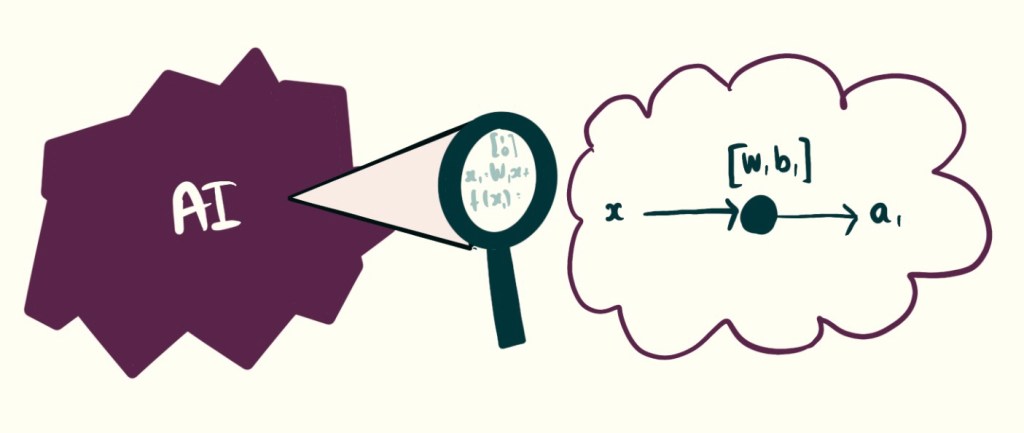
Neural networks are very large, and that makes them very complicated. But if we zoom all the way in to a single Neuron, on a single layer we can start to see what is happening. I’ll introduce just three concepts, a matrix, the weights and biases and the activation function.

For those more familiar, we will be focussing today on a single layer, single node multilayer perceptron.

If this blog is not enough, you can read more about this by searching the term Multi-layer perceptron (MLP).

Matrices Store Lots Of Numbers And Keep Their Structure

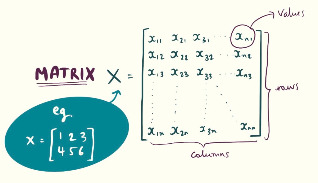
A matrix (plural matrices) is a data structure which stores numbers and preserves their structure. It’s this ability to retain structure and value that makes matrices super important.

You remember what a vector is? A column of numbers? Well a matrix is basically just many column vectors stacked together.

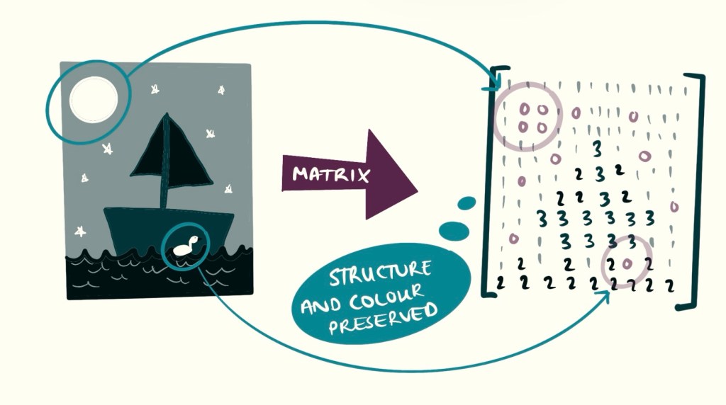
One of the best ways to understand a matrix is in the context of black-and-white images. In this case, each element in the matrix corresponds to a pixel, with the rows and columns representing the layout of the image. The value of each number determines how dark that pixel is. If you shuffle the values in the matrix, you disrupt the structure, and the image will look distorted or completely different. Changing the values again will alter the appearance once more.

In machine learning, matrices are used all the time. The weights and biases corresponding to all the nodes and layers in a neural network are stored as a matrix.

The input data that you are running through the model is also stored as a matrix. The rows in the matrix correspond to different features, and the columns correspond to different examples.

So if you remember anything, remember that matrices are used all the time, and they are just big vectors!

Weights and Biases Describe a Line of Best Fit

Now let’s go back to the neural network. We will simplify this to begin with – one layer and one neuron. In this example our data has only one feature.

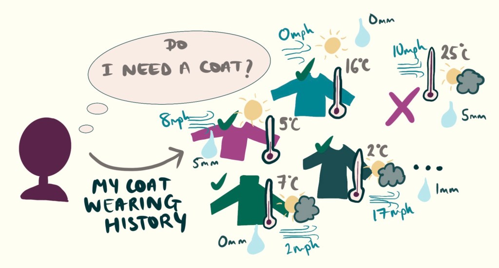
Let’s say we are trying to predict if I should wear a coat, and all I have measured is the temperature that day.

Firstly we must have a labelled training dataset. My dataset is a log of all the times I have worn a coat and the temperature it was that day.

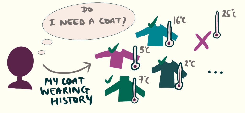
We begin by fitting a line through the training data. The parameters W and b are the parameters of this line – we try to find a good W and b such the the line Y = Wx + B models how my jumper wearing changes with temperature, based on my history.

In the future I can use my model, Y = Wx + B, and the current temperature, to decide if I need a coat!

How the parameters W and b are found is a whole new topic – Optimisation and gradient descent. I will discuss this in a later post. But for now assume these are found with a clever algorithm.

You might remember this equation from school, where W is the gradient and B is the intercept term. These define the slope and position of a straight line.

When we talk abut weights and biases, intuitively this is how they are used in a model!

So far, we’ve used just one feature—like movie length or temperature—as the input to our neuron. But real-world decisions aren’t based on just one thing.

As we start adding more layers and features, the equation becomes more complex. The variable X is no longer just temperature, it could now include wind speed, time of day, month of the year, or even rainfall. With all these additional inputs, X becomes a vector of features rather than a single number.

At this point, the simple “line of best fit” analogy doesn’t work as well, unless, of course, you can visualize in four or more dimensions.

The weights and biases are written as vectors too, or as matrices if there are multiple layers.

Great so the intuition is to fit a line of best fit through our data! Step 1 complete. ✔️

Activations Create Non-Linear Relationships

However, a straight line through a dataset might not be enough. Not all problems can be modelled with a straight line. You can have data which requires a curved line, or a wavy line. Real trends are much more complex.

So we build upon the line of best fit, and add a non-linear function. This function essentially transforms the straight line into a curved line. Adding a non-linearity enables the model to capture more complex relationships.

Adding nonlinearities to layers is a trick that ML engineers use in most of their models, typically at the end of the layer. This is called the activation function.

You can use activation functions to help build better models, and also to help encourage certain behaviours – such as outputting probabilities or keeping values within a certain bound.

Other Activation Functions Exist

Sigmoid

Squashes any input into a value between 0 and 1, like a soft yes/no decision. “Is this a cat? Yes or no?” or “Should I wear a coat?”

ReLU

Turns off if the input is negative. Otherwise, just passes the input through as-is. It is useful if you’re building deep networks. ReLU is simple, fast, and works really well in practice.

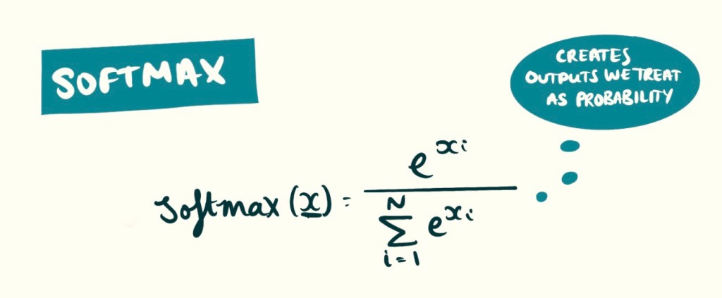
Softmax

Turns a bunch of numbers into a set of probabilities that add up to 1. You want to choose one class out of many. This example is only useful in bigger networks.

What’s Next?

We have now seen the maths! I hope it wasn’t as daunting as you might have thought. At this scale it’s relatively intuitive, and you can understand what is going on. As the model get bigger, understanding gets harder to do.

These are the foundations, and should help you appreciate what is happening under the hood.

Things we haven’t yet covered:

• How the models weights are created – a process known as Gradient Descent
• Models with more complex architectures – such as the attention mechanism, or recurrence.

So stay tuned for the next explained topic!